More Advanced Techniques

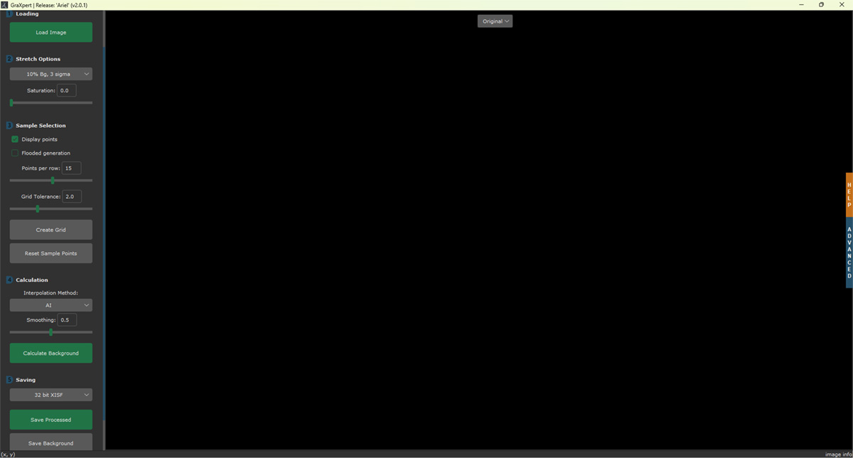
GraXpert is an excellent alternative to DBE and ABE in Pixinsight. So far I have had excellent results using this tool. It is also very simple to use. As you see from the image below, there are a number of sections in GraXpert. I will show the settings I use, but you can feel free to experiment with the tool, you might find settings that work better with your data.

Section 1 is self explanatory. Click the Load Image button, to load the image you want to correct.

Sections 2+3 I leave alone.

Section 4 I use AI as the Interpolation method. Then I click the Calculate Background button. Once the background is calculated, the button at the top middle of the screen will change from original to processed. You can also view the background extracted, by choosing Background from the dropdown on the button.

Section 5 concerns saving. If you are processing in Pixinsight, saving as a 32bit .xisf is important. Finally, save the processed file to a destination of your choosing. GraXpert will automatically choose the folder the original file came from. It will add a GraXpert extension to the filename.

To process further files, there is no need to close GraXpert, just load another image, it will close the current image automatically.

Access GraXpert From Pixinsight

In this tutorial, I will show you how to access GraXpert from Pixinsight.

GraXpert needs to be installed on your machine before undertaking this operation.

Open Pixinsight and go into Resources/Updates/Manage Repositories. Click the Add button, and paste in this URL.

https://www.ideviceapps.de/PixInsight/Utilities/

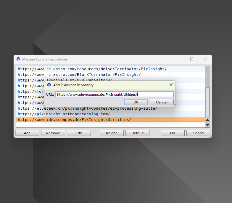
Click OK twice, then go to Resources/Updates/Check for Updates. Pixinsight will download the update for the Script. Close Pixinsight, install the update, then restart Pixinsight. Click on Script, and you will see a new folder called Toolbox. This folder contains a lot of new scripts, but the one we are interested in, is the GraXpert script. Open the script, then click on the wrench icon, locate the GraXpert.exe file, then click open. The script is now linked to GraXpert.

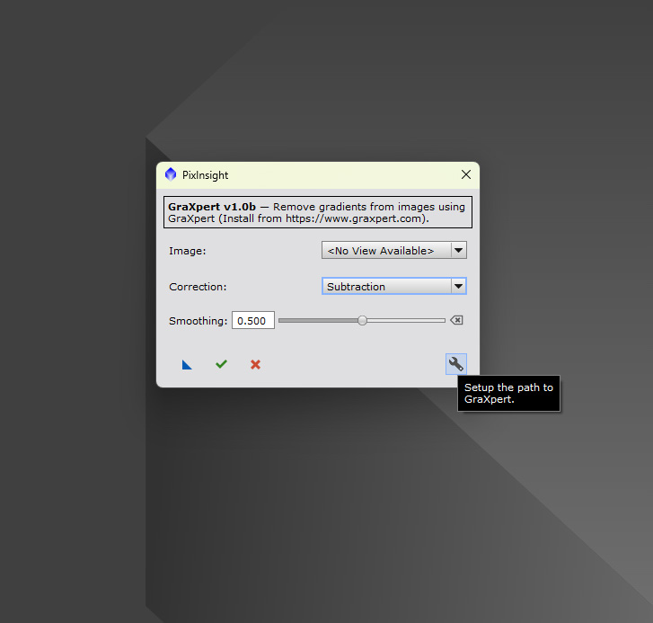
To remove the gradient from your image, open/Script/Toolbox, click on GraXpert. If you are happy with the settings, click the green tick. GraXpert will automatically remove your gradient.

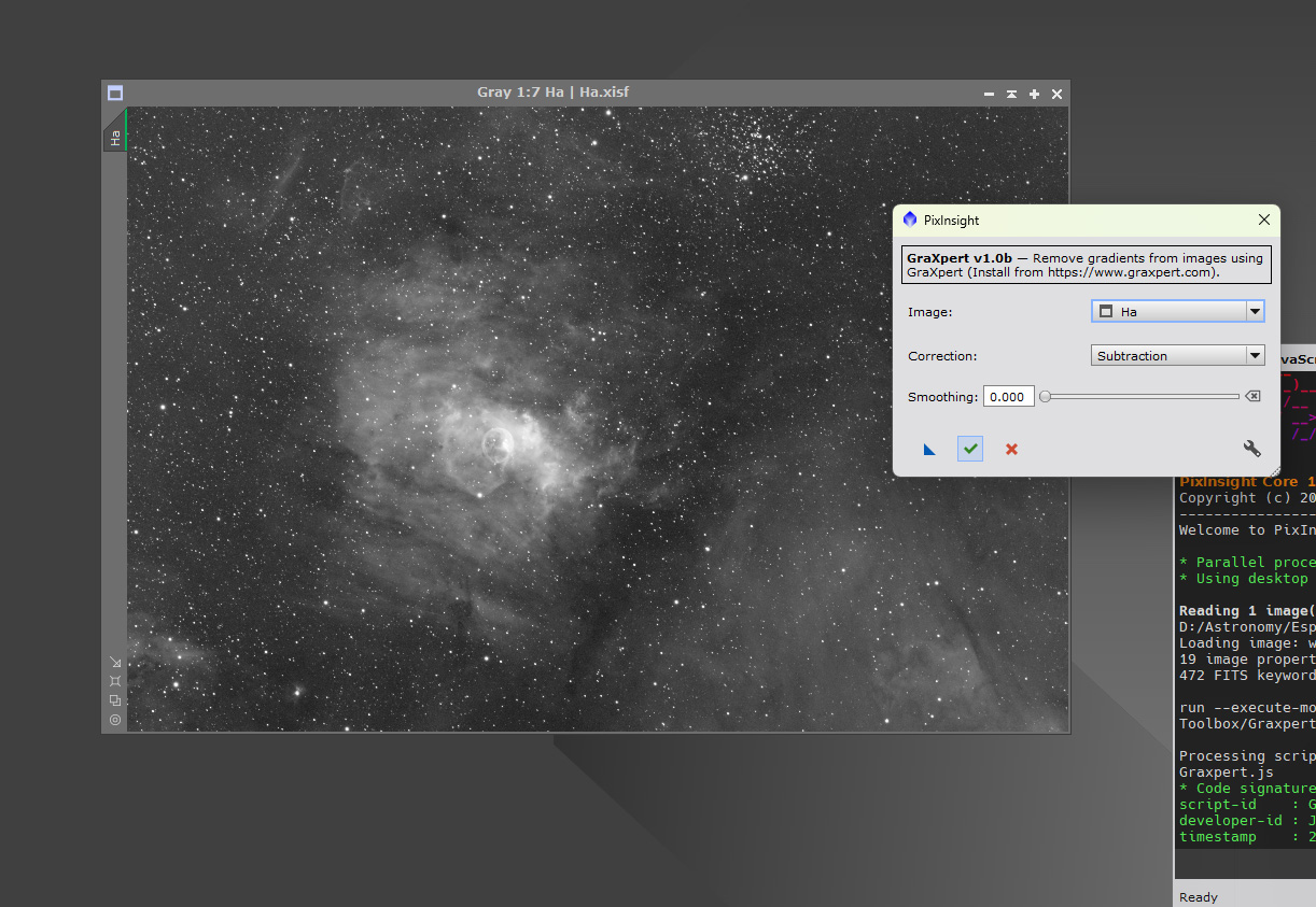
The first process after gradient removal is LinearFit. LinearFit will ensure all your stacks will have the same background median value. The reference frame is usually the stack with the darkest background.

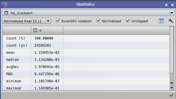
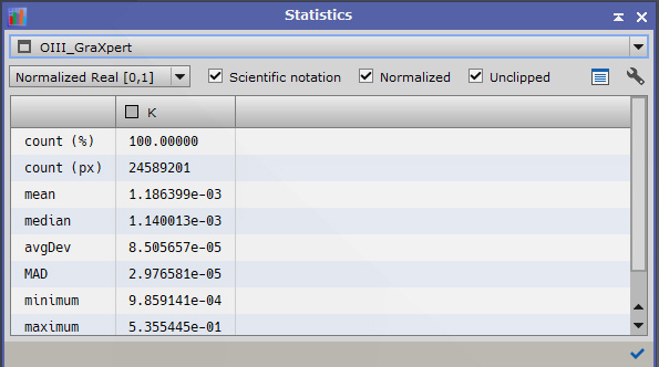
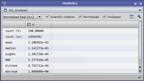
To calculate the median of an image, we use the Statistics process. Here you see I have 3 images loaded in Pixinsight, to calculate the median, I will open each stack using the dropdown box in Statistics.

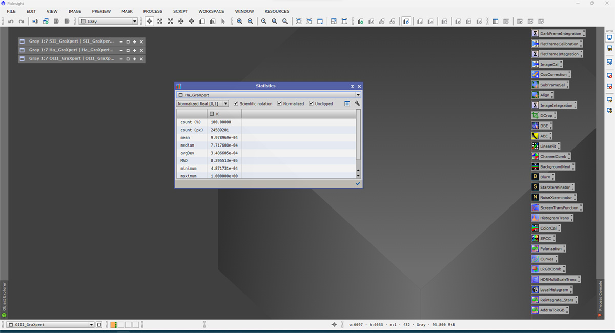
Statistics shows that the SII frame has the lowest median, so that will be our reference frame in LinearFit.

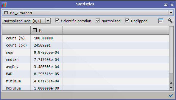
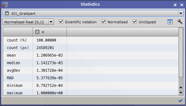
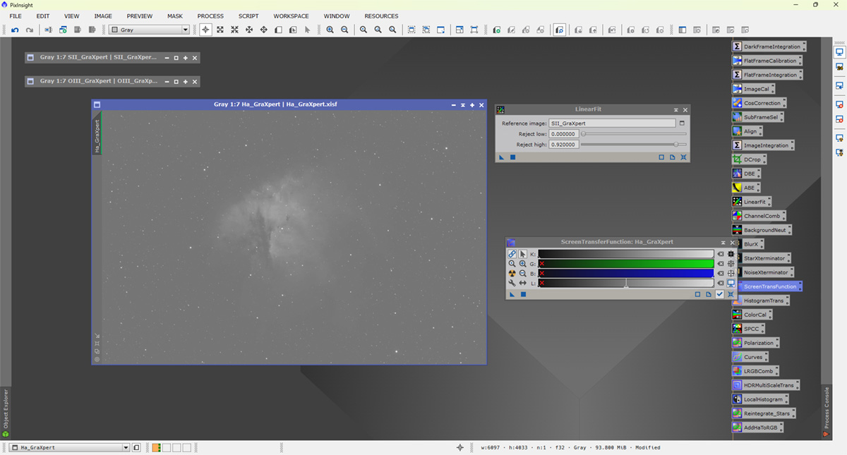
Open the LinearFit process and select your reference frame. Here you see I have chosen the SII frame as my reference. Apply LinearFit to the Ha and OIII images by dragging the blue triangle over the image. The images will probably go brighter or darker. Reset the STF by pressing Ctrl+F12, then reapply the STF, the image will return to a normal looking image.

To check LinearFit worked, we once again open the Statistics process, as we can see, all the images now have a very similar median value.

There are many ways to combine data stacks in Pixinsight, each one will give a different results.

There are also scripts available that will combine non-linear data. This method is commonly referred to as the Foraxx method, which I will cover later.

We will concentrate on using PixelMath to combine our images.

Don’t be scared of PixelMath, some astro-imagers believe you need magic powers to understand it.

When you open PixelMath, it will look like the image below.

Depending on what we are doing determines our settings. For combining SHO, first we need to uncheck the “Use single RGB/K expression” checkbox, then click the Expression editor button. This opens the Expression editor window, as seen below.

The expression editor window will show any images on the Pixinsight workspace. To make our formulae, we can either type it in, or double click the image(s) we want to use in each channel. As we are combining SHO, we use a combination of SII and Ha in the red channel.

In the green channel, we will use a combination of Ha and OIII, as seen below.

Finally, for the blue channel, we just use OIII.

To check you have no errors, click the Parse button in the bottom left. It will let you know if you have any errors in your formulae.

If no errors are found, click OK. To see all your formulae in one place, click the summary tab. 

If you are happy, we can proceed. First we Select the Create new image option. Under Color Space, we select RGB Color. To make your new combination, click the blue square. Your new image will need STF applying to it.

By adjusting the values in the Red and Green channels, we can make unlimited combinations, but remember the total value must never exceed one. Here is my combination using the formulae shown.

Here is a combination using the ChannelCombination process, (image05) you can see a huge difference immediately. The stars in the ChannelCombination are terrible.

Here is a selection of different combinations, and the values I used in PixelMath.

Image06

// R:

SII_GraXpert*.6 + Ha_GraXpert*.4

// G:

Ha_GraXpert*.5 + OIII_GraXpert*.5

// B:

OIII_GraXpert

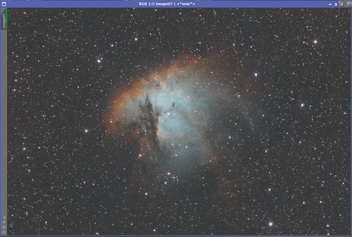
Image07

// R:

SII_GraXpert*.5 + Ha_GraXpert*.5

// G:

Ha_GraXpert*.4 + OIII_GraXpert*.6

// B:

OIII_GraXpert

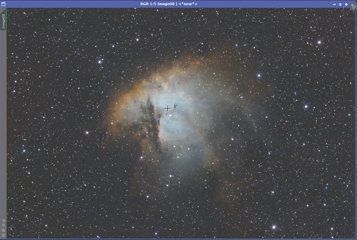
Image08

// R:

SII_GraXpert*.3 + Ha_GraXpert*.7

// G:

Ha_GraXpert*.6 + OIII_GraXpert*.4

// B:

OIII_GraXpert

Finally, the image I will use for the rest of this tutorial.

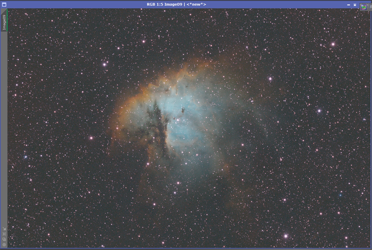
Image09

// R:

SII_GraXpert*.7 + Ha_GraXpert*.3

// G:

Ha_GraXpert*.6 + OIII_GraXpert*.4

// B:

OIII_GraXpert

We will use a different method for ColorCalibrating this image from the method shown in the Introducing Pixinsight section. For this image we will use the ColorCalibration process.

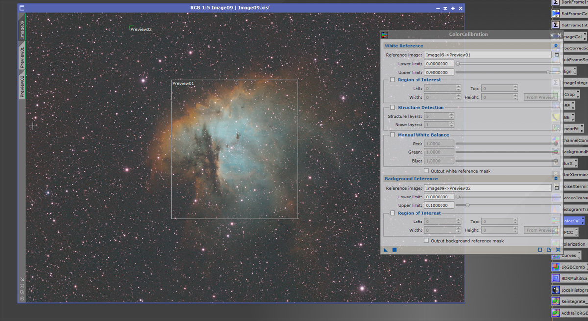
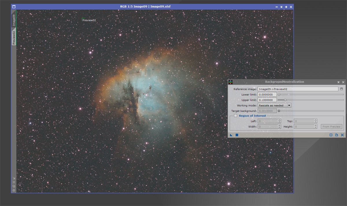
For this image, we will draw a preview around the nebula. This will be our White Reference. A second preview is drawn on the background. This will be our Background Reference.  Drag the blue triangle over the image. You will need to refresh the STF after ColorCalibration. Next we will use BackgroundNeutralization on the image. Open up BackgroundNeutralization and we can use the Background Reference preview used for the ColorCalibration. Drag the blue triangle over the image, your SHO image is now ready for the XTerminator tools. Don’t forget to refresh the STF after applying BackgroundNeutralization.

Open up BlurXterminator. For this image the default settings work fine.

Before:

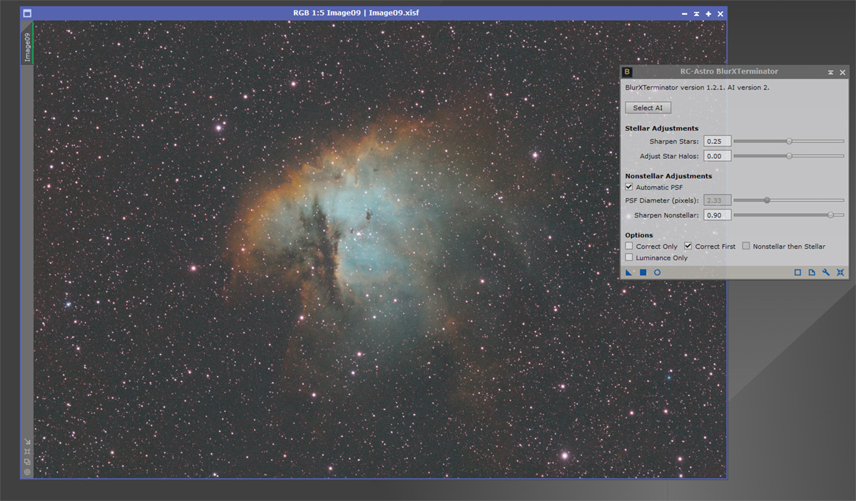
After:

Now we need to remove the stars from our image. This will make sure we don’t blow out the stars when stretching the image. Open up StarXterminator and drag the blue triangle over the image.

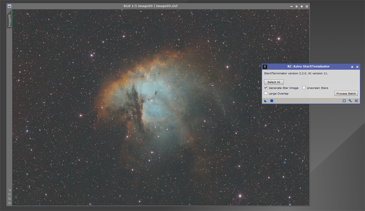
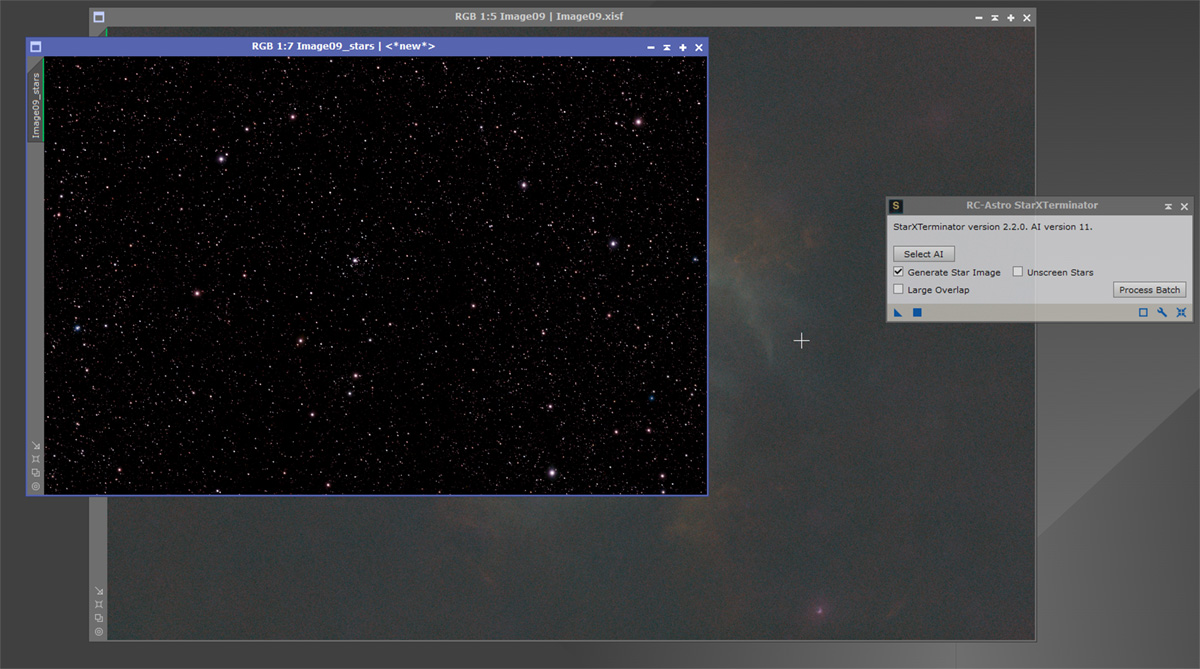
Applying the StarXterminator will result in 2 images, a starless one, and a stars image.

The next process in our list is NoiseXterminator. I dont get too aggressive with the settings. You can always reduce the noise later on.

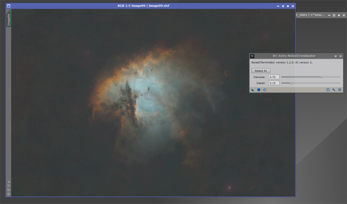
The image is now ready for stretching.

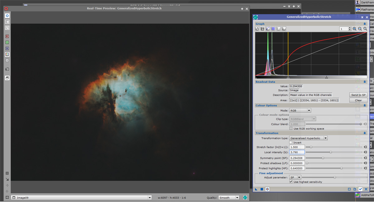
Open up GHS. The first thing we do is Reset the STF by pressing Ctrl+F12. Open a real time preview on GHS, then zoom into 250 in the graph section. This will allow you to see the curve, and to set your first symmetry point. I like to set my first symmetry point near the left edge of the curve. Hover the mouse over the curve, click once, then click send to SP. We are now ready to begin stretching.

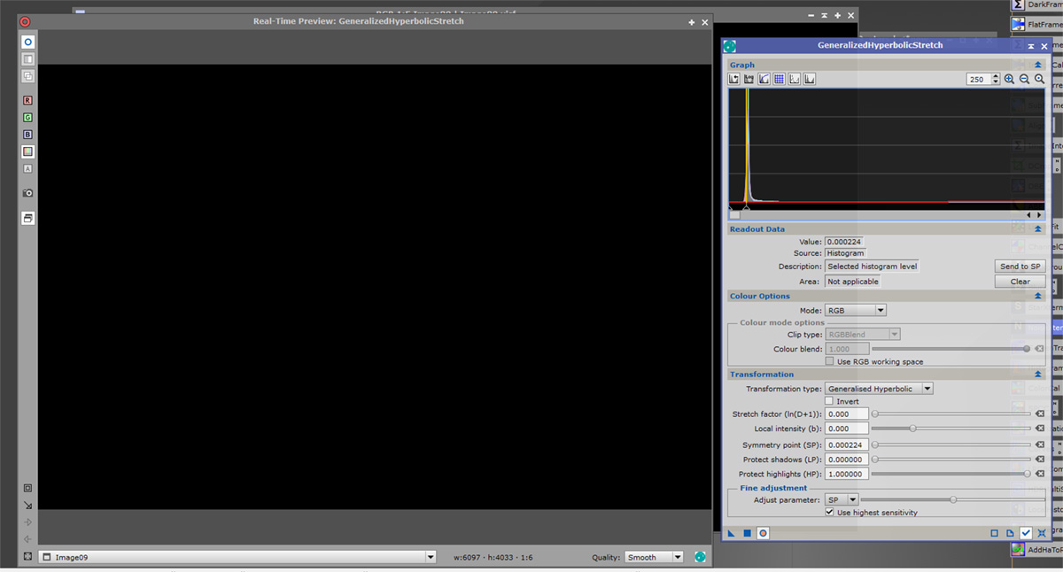
Remove the zoom level back to 1 on the graph. Start the stretching process by moving the Stretch Factor and Local Intensity sliders in the Transformation section.

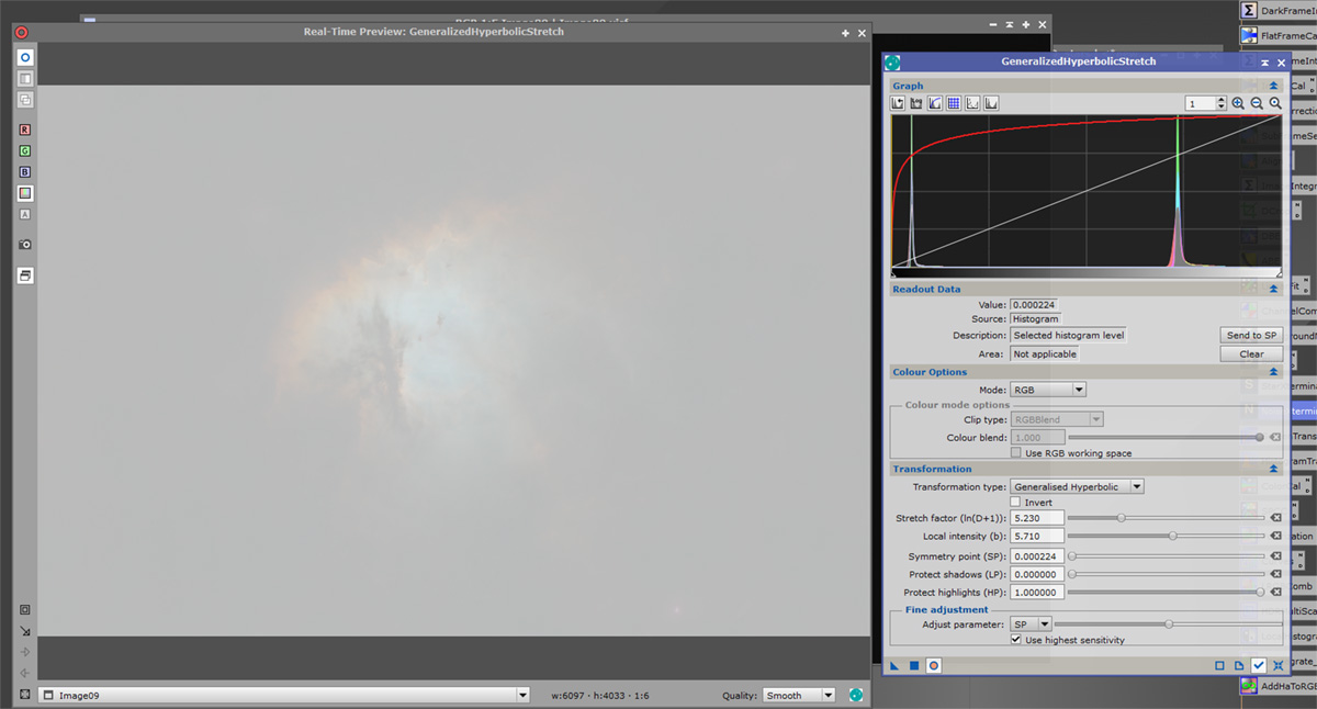
Don’t worry if your image looks horrible. Once we use the reset button on GHS, the image will look better. The image is now slightly stretched, but it needs more. My next symmetry point is selected near the middle of the curve. It is sent to SP, this time I stretch the data more conservatively.

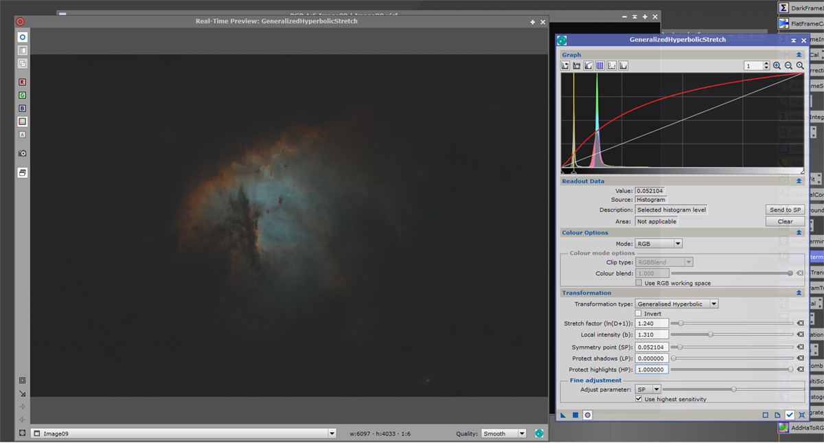
My final stretch on this image will be to increase the contrast. I will select a point to the right of the curve, and adjust the sliders until I am happy.

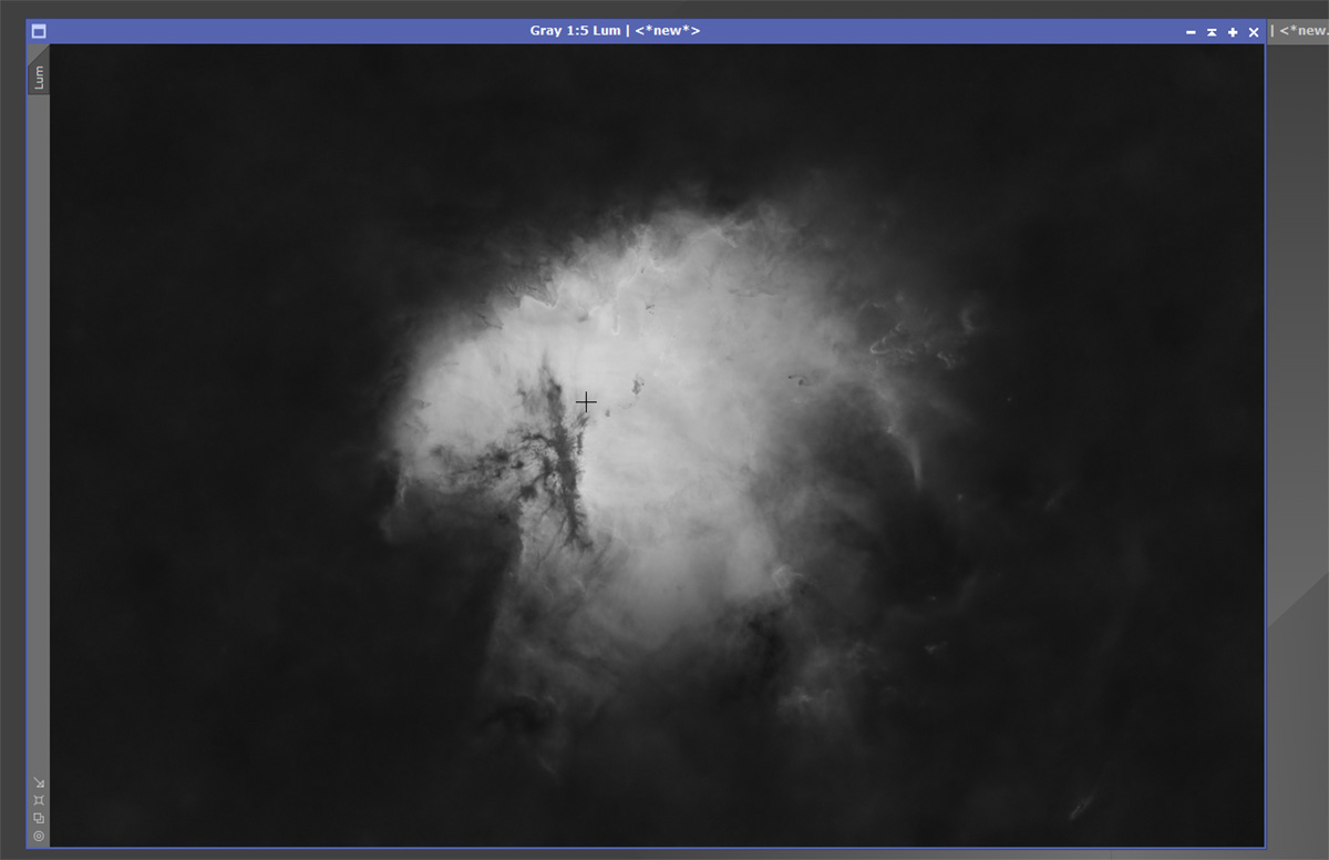
We will create a Luminance from the Ha image. The reason we create a lum file is so we can use it for the fine detail. The RGB image is basically there to provide colour information. First we make a copy of the Ha by dragging the Ha image identifier, to copy the Ha.

The next processes include applying BlurX and StarX to the Ha data. I don’t create a star image for the Lum file.

We can then apply the NoiseX to the Lum file, the then stretch in GHS. The method is exactly as the same covered in the previous chapter where we stretched the RGB data.

You should end up with a nice Lum file that can be incorporated into the RGB image. First we need to apply a few more processes to the Lum file.

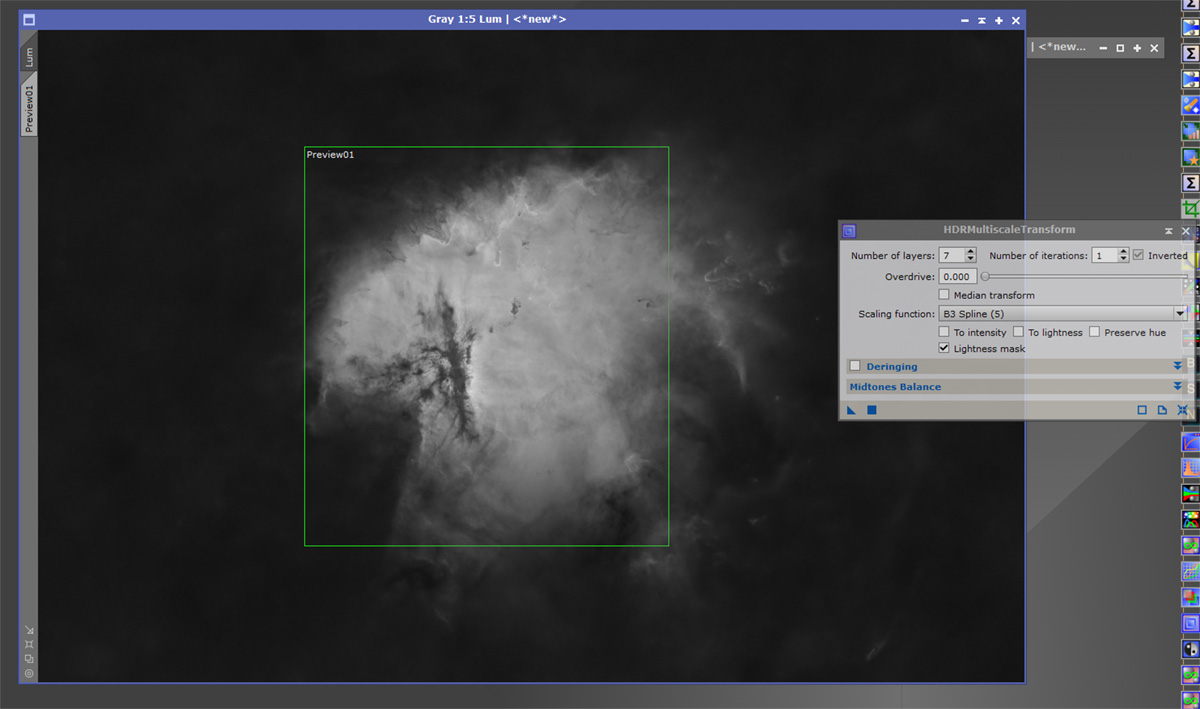
The first process we use on the Lum file is HDRMultiscaleTransform. This will reduce some of the brighter parts of the image, and bring out detail. My settings are pretty much the same for most images. Make a large preview on the image, select it, then apply the process until you are happy with the settings. With this particular image, I used 7 layers instead of my usual 6.

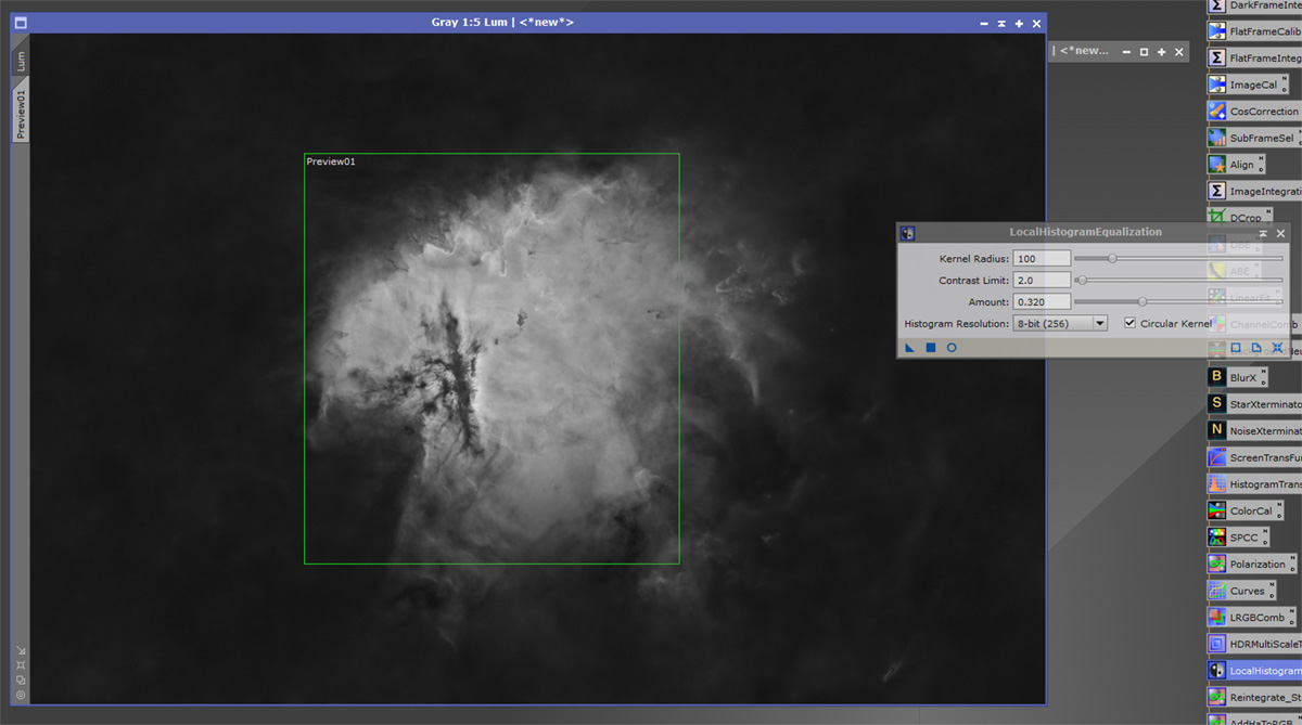
The last process we use on the Lum data is LocalHistogramEqualization. Click the real time preview button on the process, it will make it easier to see the effects your settings are having. The settings I use are more or less my default settings. Play around until you are happy. Once you are happy, press the blue square on the process.

We are now ready to combine the Lum with the RGB image. This is done by using the LRGBCombination process.

Create a large preview on the RGB image. Now uncheck the RGB boxes on the process, and select your Lum file in the appropriate box. Simply drag the blue triangle on to the RGB preview. If you are not happy, the brightness and saturation can be adjusted. Beware the brightness and saturation sliders work in the opposite way you would expect. When you are happy, apply the settings to the full image.

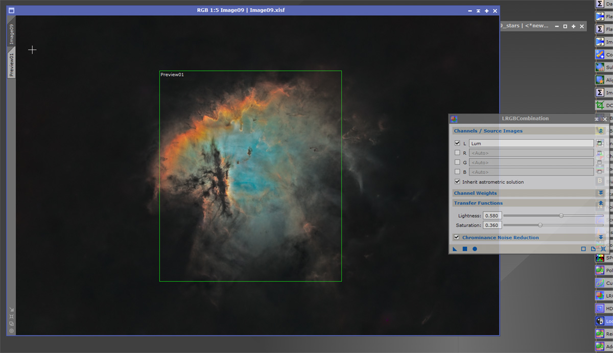
The last thing to do in Pixinsight is stretch the stars and reintegrate them.

I stretch the stars using the HistogramTransformation process until I’m happy with the stars. I apply a good helping of saturation using the curves process. Finally I rename the file to stars, and the RGB file to starless. (Very important).

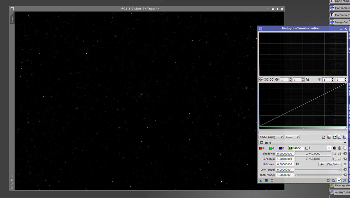
The stars are reintegrated using a Pixelmath formula. You can copy and save the formula as an icon. Press the blue square on the PixelMath formula to apply it. You will have a beautiful new image to add to your collection.

The final image should be saved as a 32 bit xisf file, and a 16 bit Tiff file, for further tweaking in Photoshop.

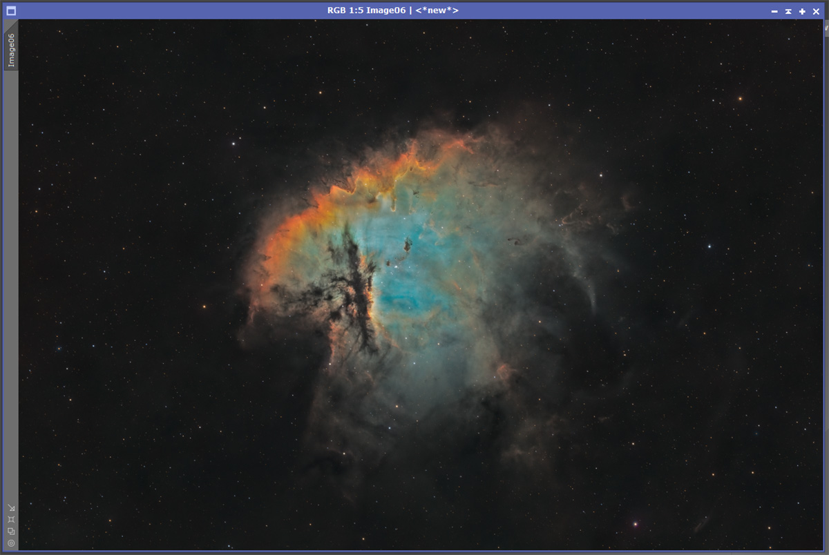
Image Annotation

There is on final thing we can do to our processed images, and that is to annotate them. This is a straightforward process in Pixinsight, but adds interest to an image.

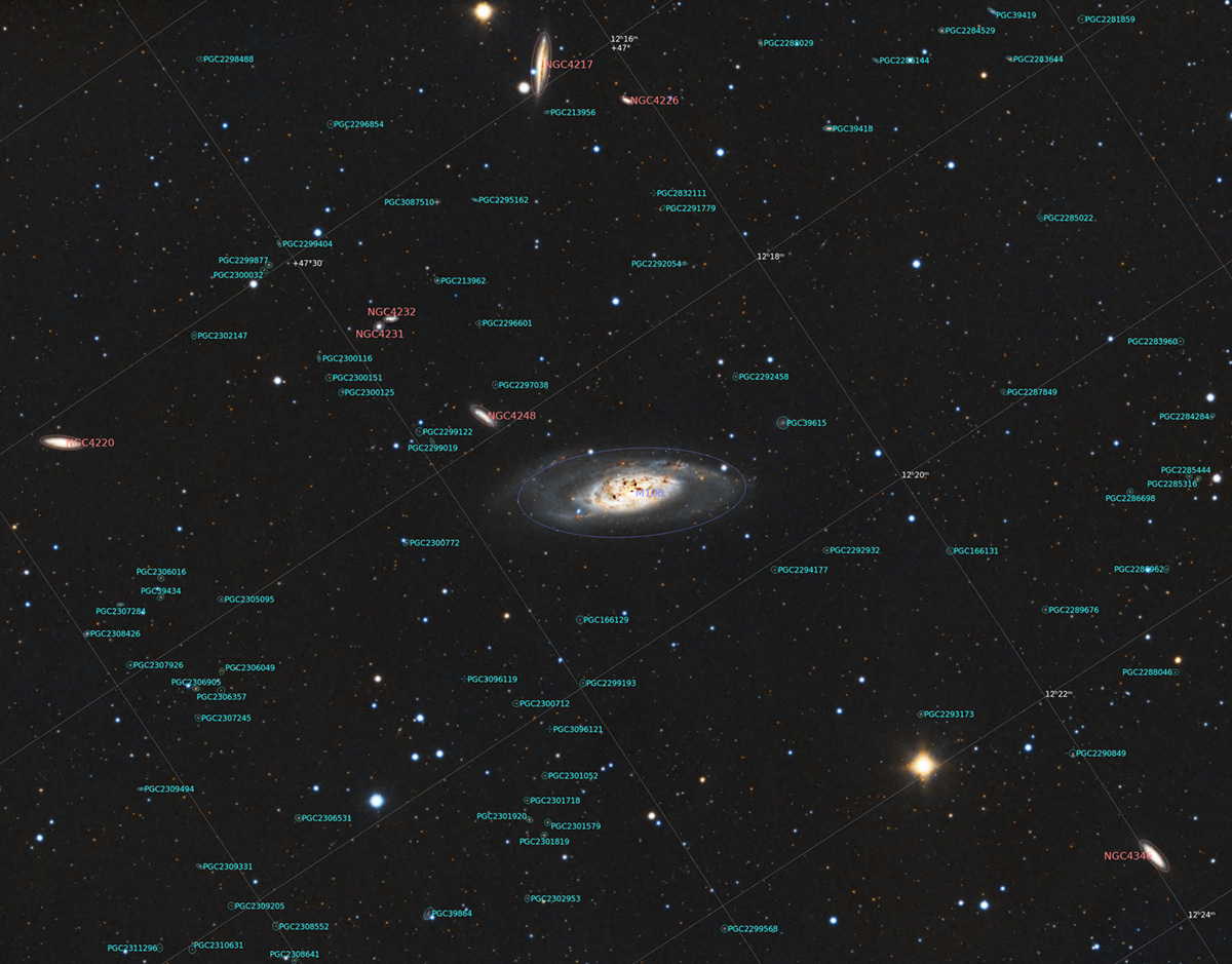
For this tutorial I will use an image of M106, which has a lot of small galaxies in the background.

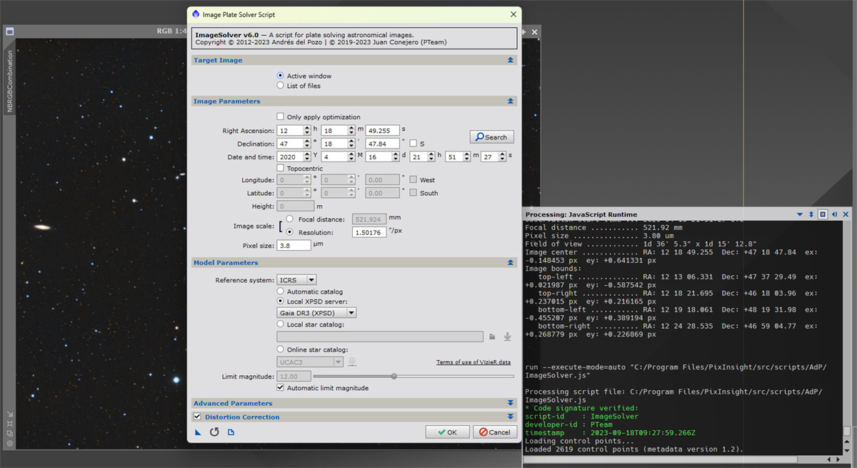
Once our image is open, preferably an xisf file, we have to open the Image Solver script, as shown in the above image. The script should read the data it needs to solve the image from the fits header. If not, click on the search box, fill in the target name. Select one of the results, press OK twice and let the script does it’s work.

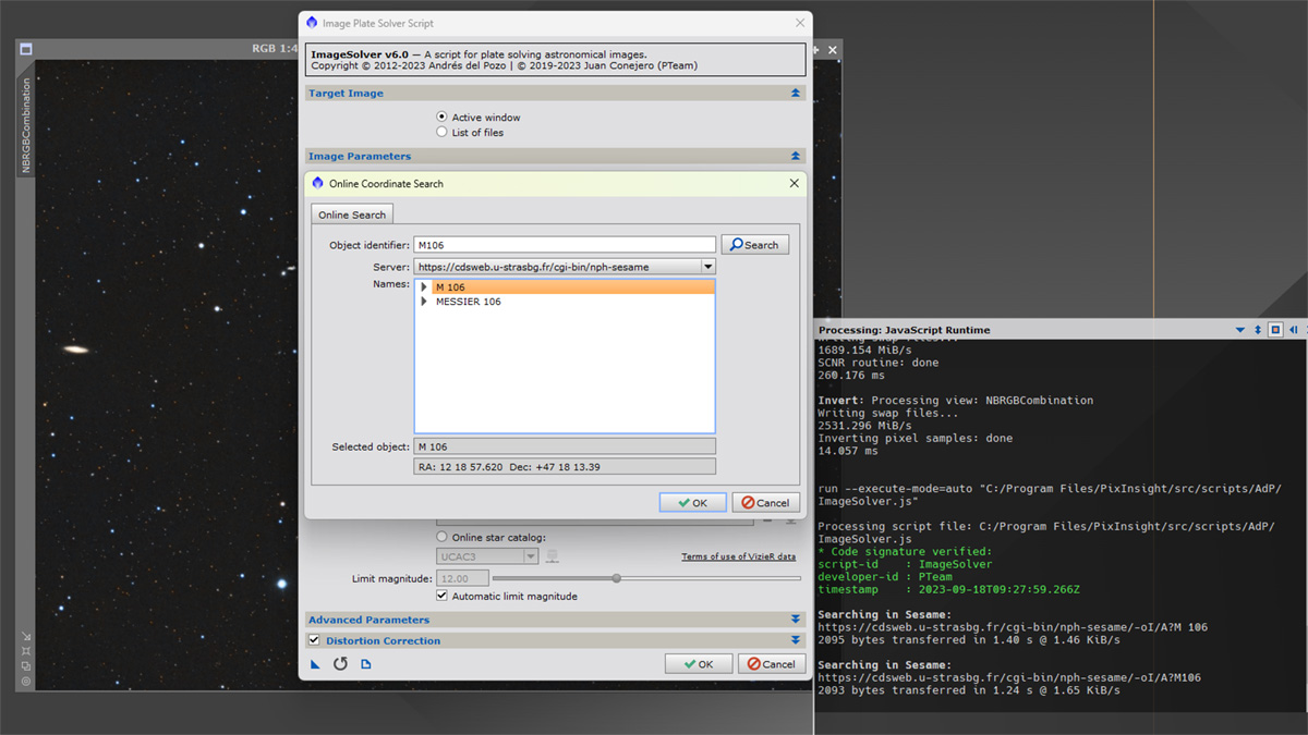
If no errors appear, we can now annotate the image. To annotate our image, we need to open the script which is found under, Script/Render/AnnotateImage

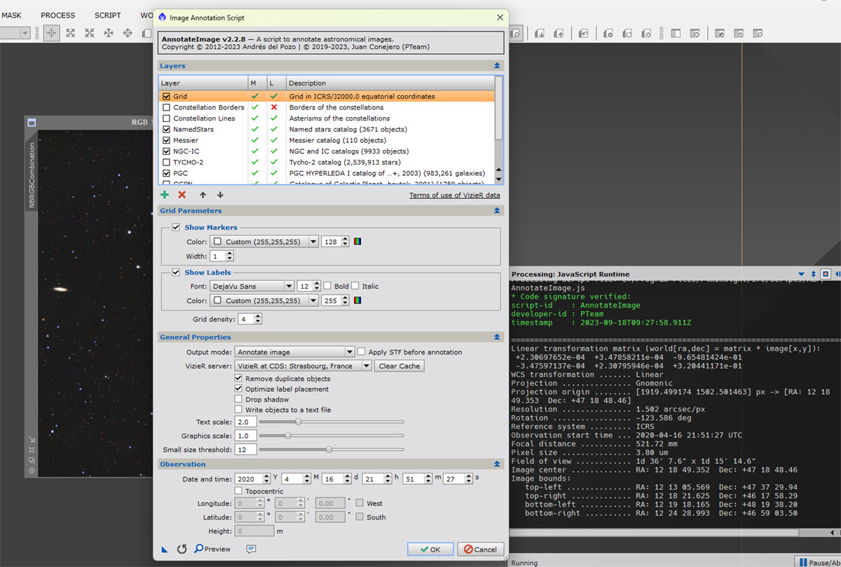
The AnnotateImage script works well with the default settings. If your image contains a lot of fuzzies, enabling the PGC checkbox will help identify them. The end result will be a new image which can be saved as an xisf file or a TIFF.